Experimental-station

experimental-station

Principle of the XAS Technique

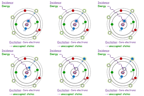
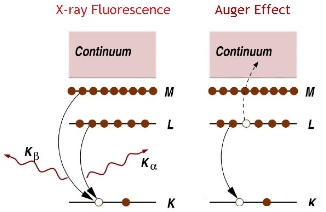
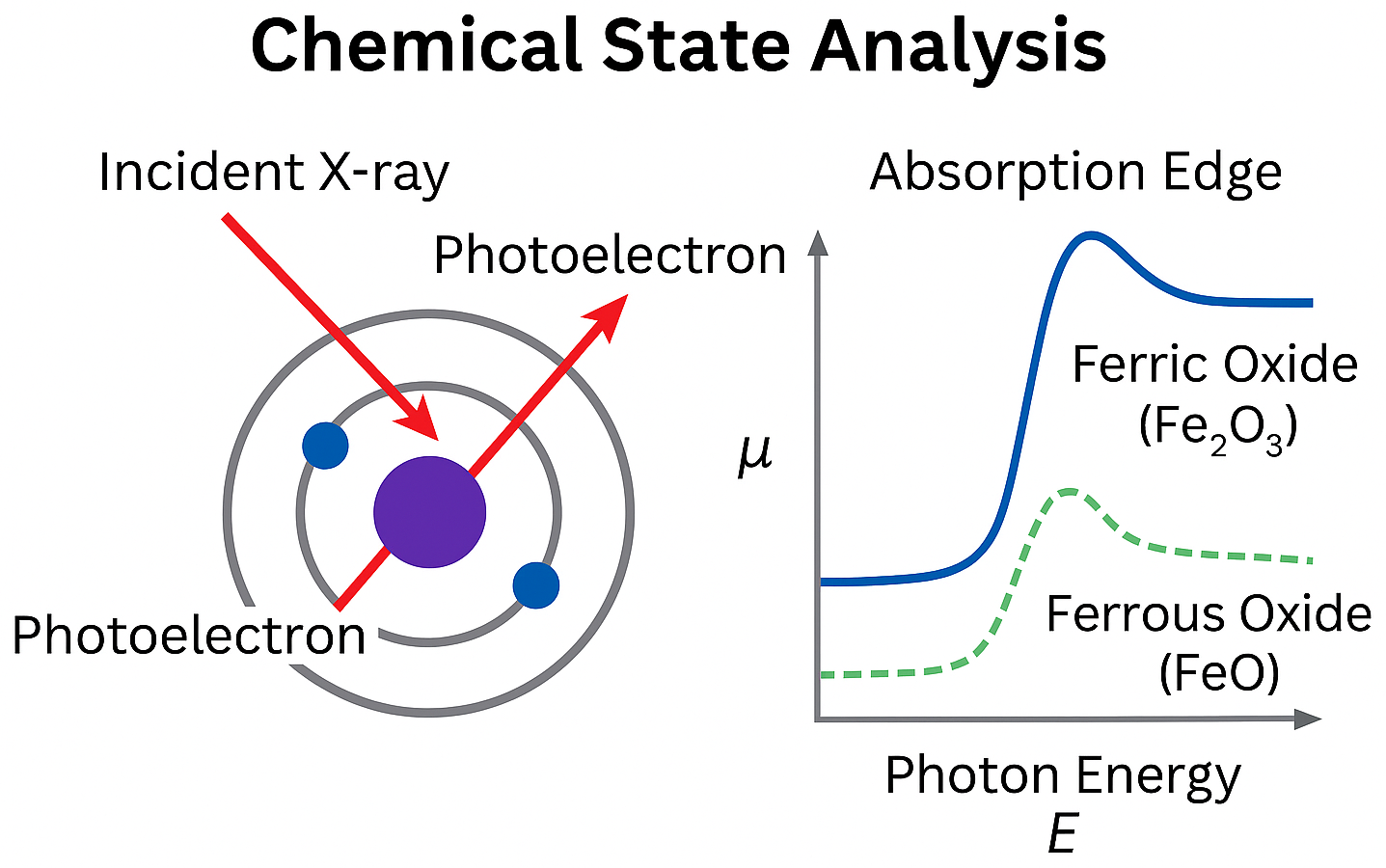
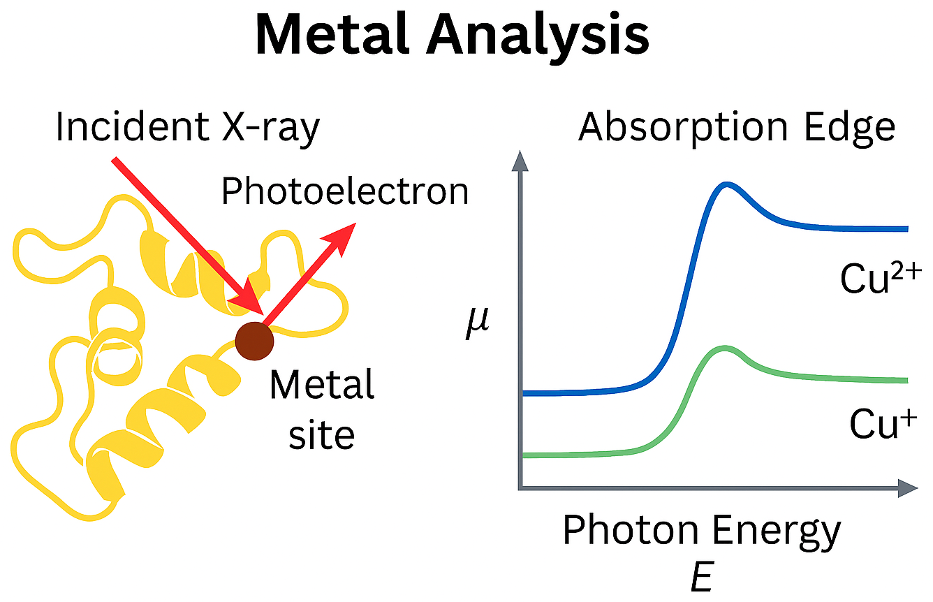
X-ray Absorption Spectroscopy (XAS) is a technique that measures how a material absorbs X-rays as a function of photon energy. When the incident X-ray energy is scanned across the absorption edge of an element in the sample, the absorption coefficient changes due to electronic transitions from core levels to unoccupied states.

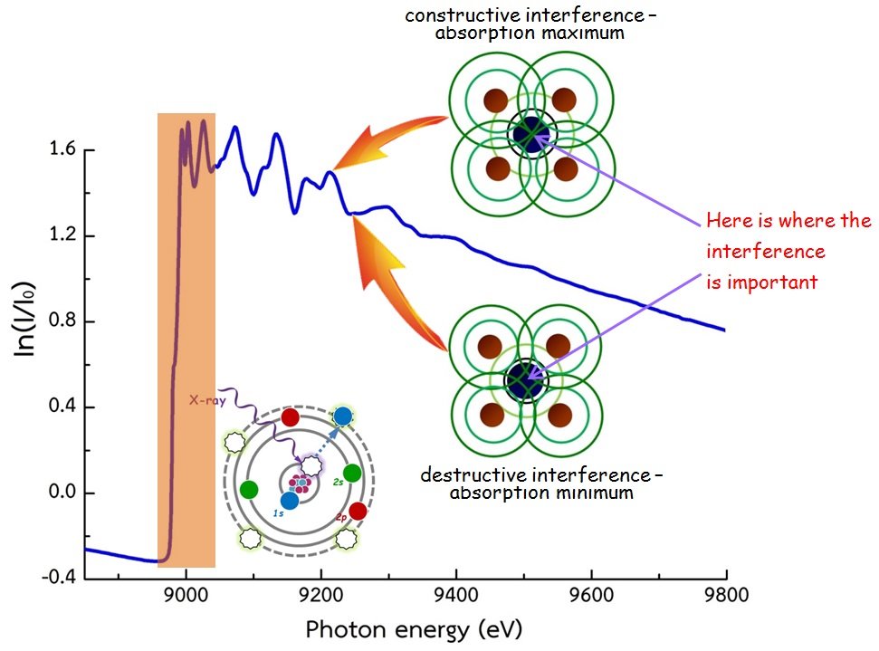
As the X-ray energy reaches the binding energy of a core electron, a sharp increase in absorption known as the absorption edge occurs. The fine structures before and after the edge arise from interactions between the photoelectron and the surrounding atomic environment. These features are divided into two regions:

XANES (X-ray Absorption Near Edge Structure): Sensitive to oxidation state, coordination geometry, and electronic structure.
EXAFS (Extended X-ray Absorption Fine Structure): Contains oscillatory features caused by photoelectron scattering, allowing determination of local atomic distances, coordination numbers, and disorder around the absorbing atom.

XAS can be measured in different detection modes, such as transmission and fluorescence, depending on sample thickness, concentration, and experimental conditions.

Fig. 1 Diagram of the photoelectric effect, fluorescence, and Auger processes — Fig. 1 Diagram of the Photoelectric Effect, Fluorescence, and Auger Processes.

Fig. 2 Schematic of XAS including pre-edge, XANES, and EXAFS regions — Fig. 2 Schematic of XAS including the pre-edge, XANES, and EXAFS regions.

The DCM is a double-crystal monochromator with a fixed beam exit. It consists of two crystals: the first (upper) crystal selects the X-ray energy, while the second (lower) crystal reflects the beam at the Bragg angle of the crystal plane so that the outgoing X-ray beam is parallel to the incoming beam. The position of the outgoing X-ray beam is approximately 3 cm lower than the incoming beam. The crystal set is selected according to the desired energy. After that, the monochromatic X-ray beam is delivered to Experimental Station 8.

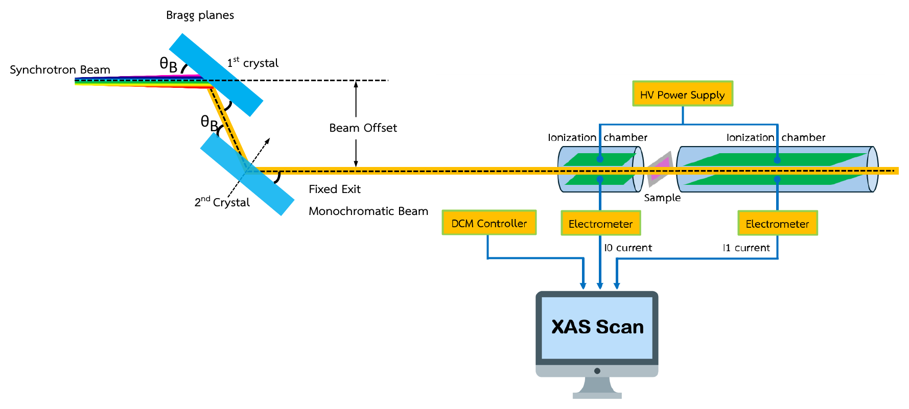
Fig. 3 Schematic diagram of the XAS measurement and experimental setup of BL8 — Fig. 3 Schematic diagram of the XAS measurement and experimental setup of the BL8 beamline.

In a transmission-mode XAS experiment, the intensities of the incident and transmitted X-rays are measured before and after the sample, referred to as I₀ and I₁, respectively. These X-ray intensities are recorded as electrical currents read by an electrometer. Both I₀ and I₁ are functions of the incident photon energy E and are related by Equation (1):

I₁(E) = I₀(E) e^−µ(E)x (1)

where µ and x represent the X-ray absorption coefficient and the sample thickness, respectively. The photon energy (E) is varied by rotating the DCM, and for each photon energy, the values of I₀(E) and I₁(E) are recorded. These values are then used to solve Equation (1) to obtain the absorption coefficient, which is known as the XAS spectrum.

µ(E)x = ln(I₀/I₁) (2)

Principle of the XFI Technique

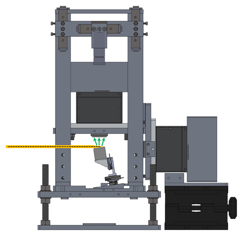
X-ray Fluorescence Imaging (XFI) is an analytical technique that combines the principles of X-ray fluorescence with spatially resolved detection to visualize elemental distributions within a sample. When a sample is irradiated by an X-ray beam, atoms absorb the incident photons and emit characteristic fluorescence X-rays. These emitted X-rays are detected and analyzed to identify the elements present and their spatial arrangement.

Key theoretical aspects

Element-specific fluorescence: Each element emits X-rays at unique energies corresponding to its electronic structure.
Non-destructive analysis: XFI does not alter or damage the sample, making it suitable for sensitive materials.
Spatial resolution: Achieved by either scanning a focused beam across the sample (micro-beam XFI) or using a full-field detector to capture the entire area simultaneously (full-field XFI).
Detection system: Energy-dispersive detectors (e.g., pnCCD) record both the position and energy of each photon, enabling multi-element imaging.

Fig. 4 Schematic diagram of the FXI station at BL8 — Fig. 4 Schematic diagram of the FXI station at the BL8 beamline.

Components of the Experimental Station

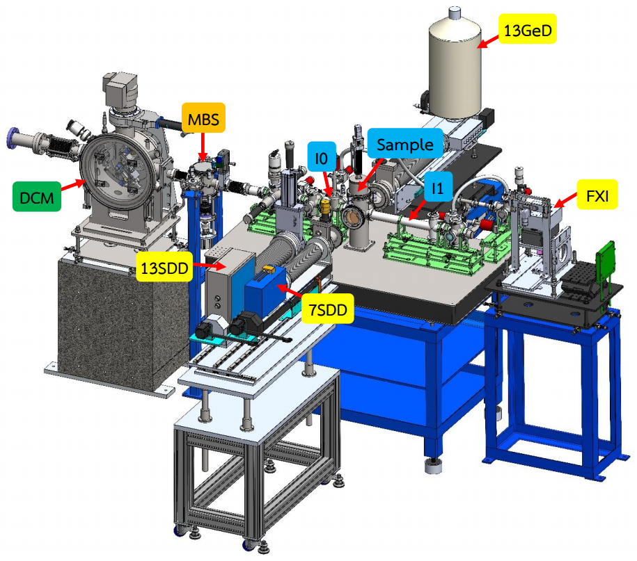
3D view of the BL8 experimental station with labelled components (DCM, MBS, I0, I1, 7SDD, 13SDD, 13GeD, FXI)

The structure of the XAS experimental station at BL8 consists of:

Ionization Chamber (I0, I1): An instrument for measuring the intensity of X-rays.
Sample Chamber (SC)
Solid State Detectors (two systems)
- Si-drift detectors (SDD): 7-element and 13-element
- 13-element Ge detector
Electrometer: An electronic device for measuring electric current.
HV Power Supply (High Voltage Power Supply)
Rough Vacuum Equipment (RV)

Sample chamber: When working at the Ti K-edge and below, purge the sample chamber with He. Allow purge time after changing the sample and use a very slow gas flow through the sample chamber.

	TM-mode	FL-mode
Detector	10-cm long ion chamber and 40-cm long ion chamber	7-element Si drift detector (7SDD) active area 7 × 65 mm²; collimator 7 × 50 mm² 13-element Si drift detector (13SDD) active area 13 × 65 mm²; collimator 13 × 50 mm² Both detectors have a 12.5 µm Be window (RaySpec Ltd) 13-element germanium detector, 13GeD (Canberra, model GUL0110S) active diameter 11.3 mm; active area 100 mm²; thickness 10 mm; distance from window 5 mm; cryostat window 25 µm Beryllium
Electronics	Current Amplifier (Keithley 428) VF converter, Counter/timer (NI)	Digital X-ray processor (DXP-XMAP)

Gas Filling Schedule of BL8

Gas type and gas pressure for TM-XAS

To get a good signal-to-noise ratio, fill the I₀ and I₁ ion chambers with gas and pressure as specified in the table below.

K-edge	L₃-edge	M₅-edge	10 cm ion chamber (I₀)	40 cm ion chamber (I₁)
Mg	As, Se		6 mbar N₂	31 mbar N₂
Al	Br, Kr	Ta, W	10 mbar N₂	53 mbar N₂
Si	Rb, Sr	Re, Os	16 mbar N₂	85 mbar N₂
P	Y, Zr	Ir, Pt, Au, Hg	24 mbar N₂	132 mbar N₂
S	Nb, Mo	Tl, Pb, Bi, Po	37 mbar N₂	200 mbar N₂
Cl	Tc, Ru	Po, At, Rn, Fr	54 mbar N₂	296 mbar N₂
Ar	Rh, Pd, Ag	Ra, Ac, Th, Pa	79 mbar N₂	433 mbar N₂
K	Cd, In	U	113 mbar N₂	619 mbar N₂
Ca	Sn, Sb, Te		160 mbar N₂	872 mbar N₂
Sc	I, Xe		11 mbar Ar	61 mbar Ar
Ti	Cs, Ba		15 mbar Ar	80 mbar Ar
V	La, Ce		19 mbar Ar	104 mbar Ar
Cr	Pr, Nd		24 mbar Ar	133 mbar Ar
Mn	Pm, Sm		31 mbar Ar	170 mbar Ar
Fe	Eu, Gd, Tb		39 mbar Ar	214 mbar Ar
Co	Dy, Ho		49 mbar Ar	269 mbar Ar
Ni	Er, Tm		61 mbar Ar	335 mbar Ar
Cu	Yb, Lu		76 mbar Ar	413 mbar Ar
Zn	Hf, Ta, W		93 mbar Ar	509 mbar Ar
Ga	W, Re		113 mbar Ar	626 mbar Ar
Ge	Os, Ir		136 mbar Ar	746 mbar Ar
As	Pt, Au		165 mbar Ar	906 mbar Ar
Se	Hg, Tl		200 mbar Ar	1013 mbar Ar
Br	Pb, Bi		240 mbar Ar	1013 mbar Ar

Applications

XAS

XAS is widely applied across various scientific disciplines, including:

Materials Science: Characterizing nanomaterials, catalysts, and superconductors.
Chemistry: Determining the chemical state and bonding characteristics of elements within materials.
Biology and Environmental Science: Investigation of metal sites in proteins and enzymes, and analysis of heavy metal contamination in soil and water.
Earth Science: Studying the structure of minerals and ions in solutions.

XAS applications: chemical state analysis and metal analysis

XFI

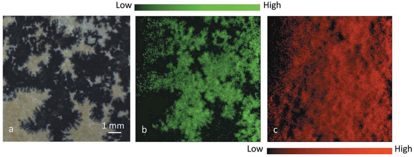
Geology: Mapping Mn distribution in dendritic limestone.
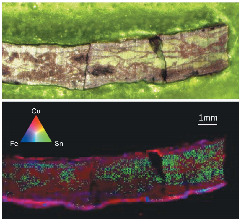
Archaeology: Investigating Sn and Cu segregation in ancient bronze.
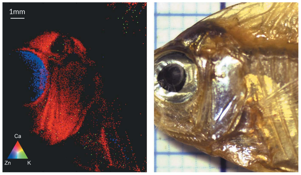
Biology / Food Science: Analyzing Zn in fisheyes and Ca in fish bones.

XFI examples: Mn in dendritic limestone, Cu/Sn/Fe in ancient bronze, Ca/Zn/K in fish